In this project, we will use K-means clustering to sort of predict an NBA player’s position based on their height and weight. For more detailed descriptions and codes, check out the Google Colab notebook of this project to learn more.

1. Project Setup

Based on NBA players’ heights and weights, we will use K-means clustering to determine whether players can be grouped into position-based clusters. (k = 3 for guard, forward, center; k = 5 for PG, SG, SF, PF, C).

2. Data Preparation

For this project, we will use the NBA Player Data (1996-2024) dataset from Kaggle. This dataset provides the height and weight of individual NBA players (as well as other stats, which we will not use in this project.). As there is no label, an unsupervised learning algorithm such as K-means clustering can come in handy.

Data cleaning

Firstly, it might be useful to visualize the raw data as a scatterplot. We will do this again after our model has clustered the data.

import matplotlib.pyplot as plt

plt.scatter(df['player_height'], df['player_weight'])
plt.xlabel('Height (cm)')
plt.ylabel('Weight (kg)')
plt.show()

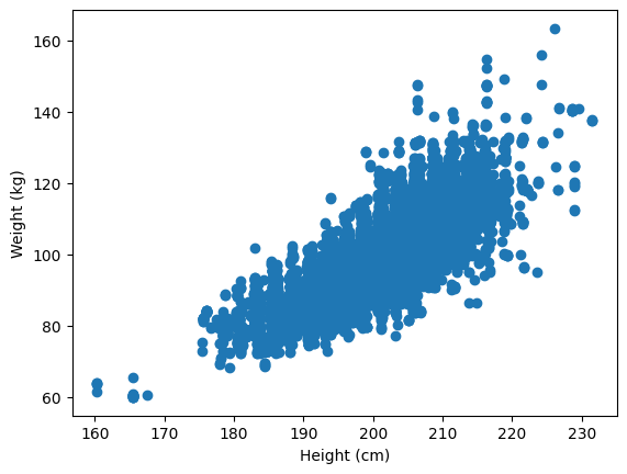
From this plot, we can see that the clusters aren’t visually obvious, and there are possible outliers (players below 170 cm).

WARNING

As I am writing this blog post, I realized that I did not address the outliers at all. One way you can deal with this is simply by removing them (some common thresholds are samples that are at least 3 standard deviations from the means or the IQR rule). Another way is to treat them like missing data and impute them.

This dataset does not have any empty values, so this is not an issue. However, since height and weight have different scales, we want to rescale them so that one feature doesn’t weigh (no pun intended) more than the other. In this case, I prefer standardization to normalization because K-means clustering uses Euclidean distance, which is sensitive to variance, and standardization preserves the variance of the data.

from sklearn.preprocessing import StandardScaler

scaler = StandardScaler()
scaled_df = pd.DataFrame(scaler.fit_transform(df), columns=df.columns)

Now, using scaled_df.describe(), we should see that the scaled data has a mean of 0 and a standard deviation of 1.

3. Modeling

Implementing a K-means clustering model is quite straightforward. Here, we will use KMeans from sklearn.cluster.

from sklearn.cluster import KMeans

model = KMeans(n_clusters=3)
model.fit(scaled_df)

Now we can visualize the clusters labeled by our model.

import seaborn as sns

sns.scatterplot(x=df['player_height'], y=df['player_weight'], hue=model.labels_)
plt.xlabel('Height (cm)')
plt.ylabel('Weight (kg)')
plt.show()

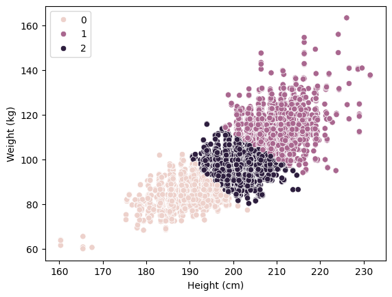
Based on typical height and weight ranges, we can infer that cluster 0 likely represents guards, 1 represents forwards, and 2 represents centers. You can try and see if these results would correctly categorize your favorite NBA player’s position or not! Just like with the linear regression model, this model also does not do well with Giannis. Maybe he’s just a one-of-a-kind player :)

4. Final Words

While you’re here, this is part 2 of a machine learning project series where I apply every machine learning algorithm I learned to an NBA-related project. If you want to check out more similar projects, look around my blog and stay tuned for more!